Imports

using LyoPronto

NonlinearSolve and TransformVariables are used for parameter fitting

using NonlinearSolve
using TransformVariables

CSV and TypedTables load and store experimental data

using TypedTables, CSV

Plots is a frontend to several plotting packages, defaulting to GR

using Plots

# All we need from StatsPlots is the @df macro
using StatsPlots: @df

# Latexify helps with LaTeX formatting in plots
using Latexify
using LaTeXStrings
# Set a default for Latexify labels
set_default(labelformat=:square) # Latexify, not Plots

Load process data

The process data here are from an actual microwave-assisted lyophilization cycle. Since thermocouples cannot be used in a microwave field, the product temperature measurements (from fiber optic probes) are in a separate file, and we must take care to synchronize the time.

As in the other examples, the file locations here are wonky in order to execute this documentation remotely; to follow along, adjust the file paths to match your local setup.

filesdir = joinpath(@__DIR__, "..", "..", "example")

dat1 = CSV.read(joinpath(filesdir, "2023-03-02_RF_Mannitol_temperature.csv"), Table)
dat2 = CSV.read(joinpath(filesdir, "2023-03-02_RF_Mannitol_process.csv"), Table,
    comment="#", stripwhitespace=true, dateformat="mm/dd/yyyy H:M:S")

To follow along, you can use the same data files here and here.

time1 = dat1.var"Elapsed [s]"

lyo_full_pre = map(dat2) do row
    nt = (tstamp = row.Timestamp,
          pch_sp = row.var"SPLYO.VACUUM_SP.F_CV"*u"mTorr",
          pch_pir = row.var"SPLYO.CHAMBER_PIRANI.F_CV"*u"mTorr",
          pch_cm = row.var"SPLYO.CHAMBER_CM.F_CV"*u"mTorr",
          Tsh_sp = row.var"SPLYO.SHELF_SP.F_CV"*u"°C",
          Tsh_i = row.var"SPLYO.SHELF_INLET.F_CV"*u"°C",
          Tsh_o = row.var"SPLYO.SHELF_OUTLET.F_CV"*u"°C",
    )
    return nt
end
time2 = uconvert.(u"hr", lyo_full_pre.tstamp .- lyo_full_pre.tstamp[1])
lyo_full = Table(lyo_full_pre; t=time2)

Table with 8 columns and 1200 rows:
      tstamp               pch_sp   pch_pir     pch_cm      Tsh_sp   Tsh_i    ⋯
    ┌──────────────────────────────────────────────────────────────────────────
 1  │ 2023-03-02T14:01:00  0 mTorr  1047 mTorr  2100 mTorr  17.4 °C  17.0 °C  ⋯
 2  │ 2023-03-02T14:02:00  0 mTorr  1047 mTorr  2100 mTorr  16.9 °C  16.5 °C  ⋯
 3  │ 2023-03-02T14:03:00  0 mTorr  1047 mTorr  2100 mTorr  16.4 °C  16.1 °C  ⋯
 4  │ 2023-03-02T14:04:00  0 mTorr  1047 mTorr  2100 mTorr  15.9 °C  15.8 °C  ⋯
 5  │ 2023-03-02T14:05:00  0 mTorr  1047 mTorr  2100 mTorr  15.4 °C  15.3 °C  ⋯
 6  │ 2023-03-02T14:06:00  0 mTorr  1047 mTorr  2100 mTorr  14.9 °C  14.9 °C  ⋯
 7  │ 2023-03-02T14:07:00  0 mTorr  1047 mTorr  2100 mTorr  14.4 °C  14.4 °C  ⋯
 8  │ 2023-03-02T14:08:00  0 mTorr  1047 mTorr  2100 mTorr  13.9 °C  14.0 °C  ⋯
 9  │ 2023-03-02T14:09:00  0 mTorr  1047 mTorr  2100 mTorr  13.4 °C  13.5 °C  ⋯
 10 │ 2023-03-02T14:10:00  0 mTorr  1047 mTorr  2100 mTorr  12.9 °C  13.0 °C  ⋯
 11 │ 2023-03-02T14:11:00  0 mTorr  1047 mTorr  2100 mTorr  12.4 °C  12.5 °C  ⋯
 12 │ 2023-03-02T14:12:00  0 mTorr  1047 mTorr  2100 mTorr  11.9 °C  11.9 °C  ⋯
 13 │ 2023-03-02T14:13:00  0 mTorr  1047 mTorr  2100 mTorr  11.4 °C  11.4 °C  ⋯
 14 │ 2023-03-02T14:14:00  0 mTorr  1047 mTorr  2100 mTorr  10.9 °C  10.8 °C  ⋯
 15 │ 2023-03-02T14:15:00  0 mTorr  1047 mTorr  2100 mTorr  10.4 °C  10.3 °C  ⋯
 16 │ 2023-03-02T14:16:00  0 mTorr  1047 mTorr  2100 mTorr  9.9 °C   9.9 °C   ⋯
 17 │ 2023-03-02T14:17:00  0 mTorr  1047 mTorr  2100 mTorr  9.4 °C   9.4 °C   ⋯
 ⋮  │          ⋮              ⋮         ⋮           ⋮          ⋮        ⋮     ⋱

Here we are concerned with the primary drying step, so we need to identify that.

istart_lyo_pd = findfirst(lyo_full.pch_sp .== 100u"mTorr")
lyo_pd = Table(lyo_full[istart_lyo_pd:end])
# Set start of primary drying as zero time
lyo_pd.t .-= lyo_pd.t[1]

It's a good idea at this point to plot temperatures and pressures, to make sure everything looks right.

plT = plot(lyo_pd.t, lyo_pd.Tsh_sp)
plp = plot(lyo_pd.t, lyo_pd.pch_pir, ylim=(0, 300))
plot!(plp, lyo_pd.t, lyo_pd.pch_cm)
plot(plT, plp, layout=(2,1), link=:x)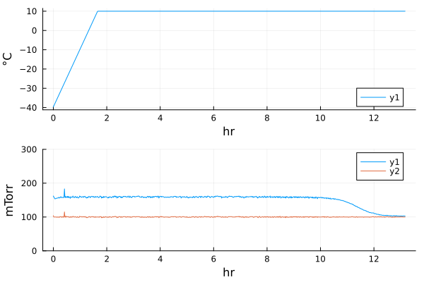

We will use this to set the shelf temperature and pressure that are used later in fitting.

Tsh = RampedVariable(uconvert.(u"K", [-40.0u"°C", 10.0u"°C"]), 0.5u"K/minute")
pch = RampedVariable(100u"mTorr")

RampedVariable(100 mTorr)

We will also need to know when primary drying actually ends, so we will use the second-derivative test in Pirani-CM convergence.

t_end = identify_pd_end(lyo_pd.t, lyo_pd.pch_pir, Val(:der2))
@df lyo_pd plot(:t, :pch_pir)
@df plot!(:t, pch_pir_sm)
tendplot!(t_end)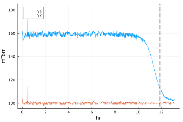

Next, we need to read the temperature data from the fiber optic probes.

thm_full = map(dat1) do row
    nt = (tstamp = row.var"Elapsed [s]"*u"s",
          T1 = row.var"T1 [C]"*u"°C",
          T2 = row.var"T2 [C]"*u"°C",
          T3 = row.var"T3 [C]"*u"°C",
          T4 = row.var"T4 [C]"*u"°C",
    )
    return nt
end
@df thm_full exptfplot(:tstamp, :T1, :T2, :T3, :T4, nmarks=40, xunit=u"hr")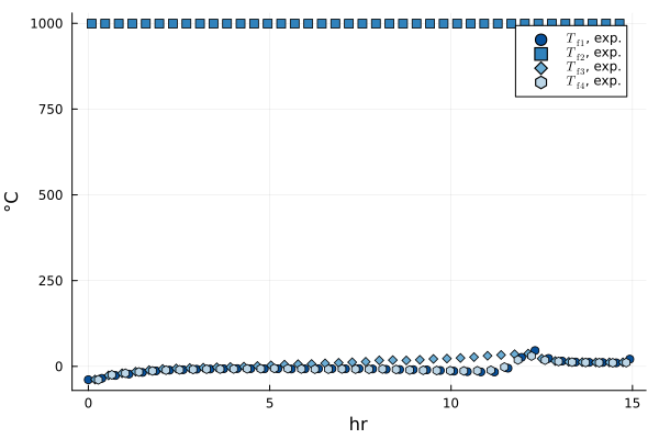

Clearly we can ignore T2, which is not reading anything physical. Also, note that one of our three remaining thermal probes is on the outside wall of a vial, while the other two are in frozen product. Based on the behavior we see in plots, it is clear that the series denoted T3 is the odd one out.

Next, we need to identify the portion of the temperature data that corresponds to primary drying. After some trial and error, I decided the following achieves that:

istart_thm_pd = argmin(thm_full.T1)
iend_thm_pd = argmax(thm_full.T4) + 600

thm_pd_sub = Table(thm_full[istart_thm_pd:iend_thm_pd])
thm_pd = Table(thm_pd_sub; t = uconvert.(u"hr", thm_pd_sub.tstamp .- thm_pd_sub.tstamp[1]))

# Plot our temperatures to make sure everything looks right
plot(u"hr", u"°C", xlabel="Time", ylabel="Temperature", size=(400,300), legend=false)
@df thm_pd exptfplot!(:t, :T1, :T4, nmarks=40)
@df thm_pd exptvwplot!(:t, :T3, nmarks=40)
plot!(Tsh, c=:black, label="shelf", tmax=13.5u"hr")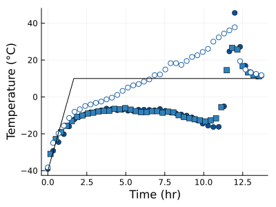

Based on that plot, we identify the part that we want to fit: everything up until the temperature minimum near 10 hours.

iend_T4 = argmin(thm_pd.T4[1000:end]) + 1000
iend_T1 = argmin(thm_pd.T1[1000:end]) + 1000
# Factor of 6 is because the temperature data are every 10 seconds,
# compared to every minute for process data
fitdat = @df thm_pd[begin:6:end] PrimaryDryFit(:t, (:T4[begin:iend_T4÷6],
    :T1[begin:iend_T1÷6]), :T3, t_end);
plot(fitdat)

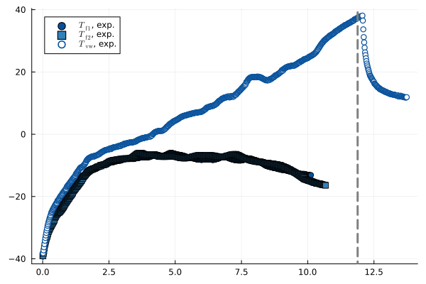
Set up other model parameters

# Vial parameters
vialsize = "6R"
rad_i, rad_o = get_vial_radii(vialsize)
A_p = π*rad_i^2  # cross-sectional area inside the vial
A_v = π*rad_o^2 # vial bottom area
m_v = get_vial_mass(vialsize)
# Formulation and fill
c_solid = 0.05u"g/mL" # g solute / mL solution
ρ_solution = 1u"g/mL" # g/mL total solution density
R0 = 1.4u"cm^2*hr*Torr/g"
A1 = 16.0u"cm*hr*Torr/g"
A2 = 0.0u"1/cm"
Rp = RpFormFit(R0, A1, A2)
Vfill = 5u"mL"
# Heat transfer
KC = 2.75e-4u"cal/s/K/cm^2"
KP = 8.93e-4u"cal/s/K/cm^2/Torr"
KD = 0.46u"1/Torr"
K_shf_f = RpFormFit(KC, KP, KD)
# Geometry
h_f0 = Vfill/A_p
m_f0 = Vfill * ρ_solution
# RF fit parameters (dummy values, will be replaced in fitting)
Bf = 2.0e7u"Ω/m^2"
Bvw = 0.9e7u"Ω/m^2"
Kvwf = 10.0u"W/K/m^2"
# Controllable inputs
f_RF = 8u"GHz"
# Total of 10W nominal power, multiplied by 0.54 to account for system losses
P_per_vial = RampedVariable(10u"W"/17 * 0.54) # actual power / vial

RampedVariable(0.31764705882352945 W)

We combine these into a ParamObjRF which will bundle up all the parameters we need. This object needs to be constructed with all these parameters in this order, so it has a constructor taking this tuple-of-tuples form that helps logical grouping.

params_base = ParamObjRF((
    (Rp, h_f0, c_solid, ρ_solution),
    (K_shf_f, A_v, A_p),
    (pch, Tsh, P_per_vial),
    (m_f0, LyoPronto.cp_ice, m_v, LyoPronto.cp_gl),
    (f_RF, LyoPronto.eppf, LyoPronto.epp_gl),
    (Kvwf, Bf, Bvw),
))

ParamObjRF{}(RpFormFit{}(1.4 hr cm^2 Torr g^-1, 16.0 hr cm Torr g^-1, 0.0 cm^-1), 0.015915494309189534 mL mm^-2, 0.05 g mL^-1, 1 g mL^-1, RpFormFit{}(0.000275 cal K^-1 cm^-2 s^-1, 0.000893 cal K^-1 cm^-2 s^-1 Torr^-1, 0.46 Torr^-1), 380.132711084365 mm^2, 314.1592653589793 mm^2, RampedVariable(100 mTorr), RampedVariable(Unitful.Quantity{Float64, 𝚯, Unitful.FreeUnits{(K,), 𝚯, nothing}}[233.14999999999998 K, 283.15 K], 0.5 K minute^-1), RampedVariable(0.31764705882352945 W), 5 g, 2090.0 J kg^-1 K^-1, 7.9 g, 839.0 J kg^-1 K^-1, missing, 8 GHz, LyoPronto.Dielectric.ϵppf, 0.024, 10.0 W K^-1 m^-2, 2.0e7 Ω m^-2, 9.0e6 Ω m^-2, missing)

Estimates of some physical properties we will often need are included in LyoPronto, including the heat capacity of ice and glass. A literature correlation for the dielectric loss of ice is provided as eppf, and for glass we provide a more-uncertain single value of epp_gl.

Parameter fitting

First, we set up the fit problem, and double check that our guess values are close-ish.

# Transform variables to map from a 3-component vector to bounded physical values
trans_KBB = KBB_transform_bounded(Kvwf, Bf, Bvw)
# Create nonlinear least-squares function
# nls_M1 = NonlinearFunction{true, SciMLBase.FullSpecialize}(nls_pd!, resid_prototype=zeros(num_errs(fitdat)))
# LyoPronto provides a shorthand for this:
nls_M1 = NonlinearFunction(fitdat)
# Guess values for fit parameters, in log space
# In practice, these often need tinkering with
p0 = [3.0, 3.0, 0.3]
# Check the physical solution for these guess values
tsol = gen_sol_pd(p0, trans_KBB, params_base)
modrftplot(tsol)
plot!(fitdat, nmarks=40)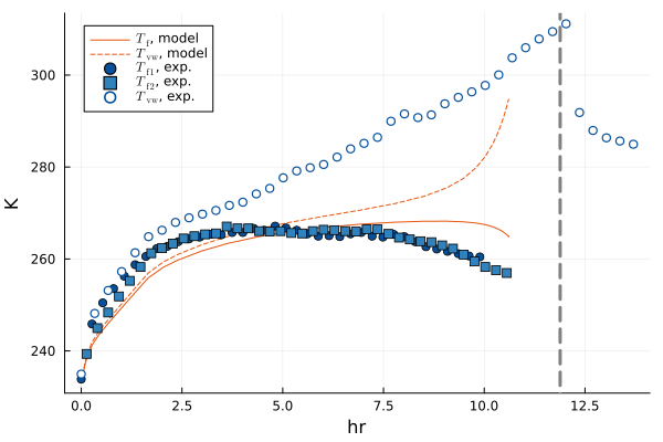

Now, we actually run the fit, which is a nonlinear least squares problem

opt1 = solve(NonlinearLeastSquaresProblem(nls_M1, p0, (trans_KBB, params_base, fitdat)), LevenbergMarquardt())
# Get the fitted solution
prof_RF = gen_sol_pd(opt1.u, trans_KBB, params_base)
# Get the fitted parameters in parameter space
transform(trans_KBB, opt1.u)

(Kvwf = 20.065286928965858 W K^-1 m^-2, Bf = 6.278992568052382e8 Ω m^-2, Bvw = 9.86594499083798e6 Ω m^-2)

Now, we can plot the fit results against the experimental data.

# Set up the plot
plT = plot(u"hr", u"°C", xlabel="Time", ylabel="Temperature")
# Experimental data
@df thm_pd exptfplot!(:t, :T4, :T1, nmarks=40)
@df thm_pd exptvwplot!(:t, :T3, nmarks=40, label=L"$T_\mathrm{vw1}$, exp.")
# Model results
modrftplot!(prof_RF, markeralpha=0, trimend=1)
# Shelf temperature
plot!(Tsh, c=:black, label=L"T_\mathrm{sh}")
# End of primary drying
tendplot!(fitdat.t_end, label="", ls=:dash)
# Mark the end of drying with a nice label
annotate!(9, -32, Plots.text("end of drying,\nRF off", 12, "Computer Modern"))
plot!([fitdat.t_end-1.5u"hr", fitdat.t_end-0.2u"hr"], [-30, -30], arrow=:arrow, c=:black, linewidth=1, label="")
# Set other plot attributes
plot!(legend=:topleft, ylim=(-40, 50), xlim=(0,13))
plot!(size=(600,400), left_margin=15Plots.px)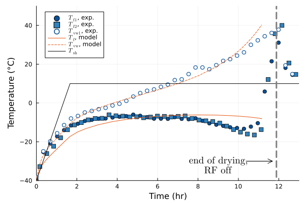

This page was generated using Literate.jl.