Optimize time-varying chamber pressure during primary drying

We need a few imports:

import matplotlib.pyplot as plt
from matplotlib import rc as matplotlibrc
from ruamel.yaml import YAML
yaml = YAML()

from lyopronto import opt_Pch, plot_styling

Then, we provide all the necessary simulation parameters.

# Set up the simulation settings
# This needs to be a dict with string keys, which can be expressed in YAML as well
sim = yaml.load("""
tool: Optimizer
Kv_known: true
Rp_known: true
Variable_Pch: true
Variable_Tsh: false
""")
# Or, equivalently:
sim = {
    'tool': 'Optimizer',
    'Kv_known': True,
    'Rp_known': True,
    'Variable_Pch': True,
    'Variable_Tsh': False}


# Vial and fill properties
vial = {
    # Av = Vial area in cm^2
    'Av': 3.80,
    # Ap = Product Area in cm^2
    'Ap': 3.14,
    # Vfill = Fill volume in mL
    'Vfill': 2.0
}

# Product properties
product = {
    # cSolid = Fractional concentration of solute in the frozen solution
    'cSolid': 0.05,
    # Product Resistance Parameters
    'R0': 1.4,  # cm^2-hr-Torr/g
    'A1': 16.0,  # cm-hr-Torr/g
    'A2': 0.0,  # 1/cm
    # Critical product temperature
    # At least 2 to 3 deg C below collapse or glass transition temperature
    'T_pr_crit': -5  # in deg C
}

# Vial Heat Transfer Parameters
ht = {
    'KC': 2.75e-4,  # cal/s-cm^2-K
    'KP': 8.93e-4,  # cal/s-cm^2-K-Torr
    'KD': 0.46      # 1/Torr
}

# Chamber Pressure bounds (optimizer will search within these)
Pchamber = {
    # min = Minimum chamber pressure in Torr
    'min': 0.05,
    # max = Maximum chamber pressure in Torr
    'max': 1000.0
}

# Shelf Temperature
Tshelf = {
    # init = Initial shelf temperature in C
    'init': -40.0,
    # setpt = Shelf temperature set points in C
    'setpt': [10.0],
    # dt_setpt = Time for which shelf temperature set points are held in min
    'dt_setpt': [1800.0],
    # ramp_rate = Shelf temperature ramping rate in C/min
    'ramp_rate': 1.0
}

# Equipment capability line
eq_cap = {
    'a': -0.182,  # slope
    'b': 11.7     # intercept
}

# Number of vials (used for equipment capability calculation)
nVial = 398

# Time step
dt = 0.01  # hr

Now, we are ready to run the optimization, which is lyopronto.opt_Pch.dry.

documentation

Here is the docstring for opt_Pch.dry:

Find optimal chamber pressures for a given lyophilization process, with fixed shelf temperatures.

Parameters:

Name	Type	Description	Default
vial	dict	Vial properties, including 'Vfill', 'Ap', and 'Av'..	required
product	dict	Product properties, including 'cSolid', 'T_pr_crit', and Rp parameters 'R0', 'A1', and 'A2'.	required
ht	dict	Heat transfer properties, including 'KC', 'KP', and 'KD'.	required
Pchamber	dict	Chamber pressure bounds between which optimizer will search.	required
Tshelf	dict	Shelf temperature set points and time (see docs).	required
dt	float	Fixed time step for output [hours]	required
eq_cap	dict	Equipment capability line, with 'a' slope and 'b' intercept.	required
nVial	int	Number of vials in the load, used for equipment capability calculation.	required

Returns:

Name	Type	Description
output_table	ndarray	Simulation output table with columns for: 0. Time [hr], 1. Sublimation front temperature [°C], 2. Vial bottom temperature [°C], 3. Shelf temperature [°C], 4. Chamber pressure [mTorr], 5. Sublimation flux [kg/hr/m²], 6. Drying percent [%]

Source code in lyopronto/opt_Pch.py

def dry(vial,product,ht,Pchamber,Tshelf,dt,eq_cap,nVial):
    """Find optimal chamber pressures for a given lyophilization process, with fixed shelf temperatures.

    Args:
        vial (dict): Vial properties, including 'Vfill', 'Ap', and 'Av'..
        product (dict): Product properties, including 'cSolid', 'T_pr_crit', and Rp parameters 'R0', 'A1', and 'A2'.
        ht (dict): Heat transfer properties, including 'KC', 'KP', and 'KD'.
        Pchamber (dict): Chamber pressure bounds between which optimizer will search.
        Tshelf (dict): Shelf temperature set points and time (see docs).
        dt (float): Fixed time step for output [hours]
        eq_cap (dict): Equipment capability line, with 'a' slope and 'b' intercept.
        nVial (int): Number of vials in the load, used for equipment capability calculation.

    Returns:
        output_table (ndarray): Simulation output table with columns for:
            0. Time [hr],
            1. Sublimation front temperature [°C],
            2. Vial bottom temperature [°C],
            3. Shelf temperature [°C],
            4. Chamber pressure [mTorr],
            5. Sublimation flux [kg/hr/m²],
            6. Drying percent [%]
    """

    ##################  Initialization ################

    # Initial fill height
    Lpr0 = functions.Lpr0_FUN(vial['Vfill'],vial['Ap'],product['cSolid'])   # [cm]

    # Initialization of time
    iStep = 0      # Time iteration number
    t = 0.0    # Time [hr]

    # Initialization of cake length
    Lck = 0.0    # Cake length [cm]
    percent_dried = Lck/Lpr0*100.0        # Percent dried

    # Initial chamber pressure: middle of range, or 2*min if only min given
    P0 = (Pchamber['min'] + Pchamber.get('max', Pchamber['min']*3))/2.0    

    # Initial shelf temperature
    Tsh = Tshelf['init']        # [degC]
    Tshelf = Tshelf.copy()
    Tshelf['setpt'] = np.insert(Tshelf['setpt'],0,Tshelf['init'])        # Include initial shelf temperature in set point array
    # Shelf temperature control time
    Tshelf['t_setpt'] = np.array([[0]])
    for dt_i in Tshelf['dt_setpt']:
        Tshelf['t_setpt'] = np.append(Tshelf['t_setpt'],Tshelf['t_setpt'][-1]+dt_i/constant.hr_To_min)

    # Initial product and shelf temperatures
    Tb0 = product['T_pr_crit'] -0.1   # [degC]
    Ts0 = Tb0 - 0.1   # [degC]
    Tsh0 = Tb0 +0.1   # [degC]

    ######################################################

    ################ Primary drying ######################
    # Objective function to be minimized to maximize sublimation rate
    def objfun(x):
        return (x[0]-x[4])
    # Exact gradient of the linear objective, so SLSQP does not
    # finite-difference it at every point.
    def objfun_jac(x):
        return np.array([1.0,0.0,0.0,0.0,-1.0,0.0,0.0])
    # Quantities solved for: x = [Pch,dmdt,Tbot,Tsh,Psub,Tsub,Kv]
    x0 = np.array([P0,0.0,Tb0,Tsh0,P0*1.1,Ts0,3.0e-4])    # Initial values
    failures = 0

    while(Lck<=Lpr0): # Dry the entire frozen product

        Rp = functions.Rp_FUN(Lck,product['R0'],product['A1'],product['A2'])  # Product resistance [cm^2-hr-Torr/g]

        # Stack the equality constraints into one vector-valued constraint so
        # SLSQP evaluates and differentiates the whole system once per point
        # rather than once per component: sublimation front pressure [Torr],
        # sublimation rate [kg/hr], vial heat transfer balance, shelf
        # temperature [degC], vial heat transfer coefficient [cal/s/K/cm^2], and fixed shelf temperature [degC]
        def eq_sys(x, Tsh=Tsh):
            return np.array(functions.Eq_Constraints(x[0],x[1],x[2],x[3],x[4],x[5],x[6],Lpr0,Lck,vial['Av'],vial['Ap'],Rp)
                            + (x[6]-functions.Kv_FUN(ht['KC'],ht['KP'],ht['KD'],x[0]), x[3]-Tsh))
        # Inequality constraints: equipment capability and maximum product temperature
        def ineq_sys(x):
            return np.array(functions.Ineq_Constraints(x[0],x[1],product['T_pr_crit'],x[2],eq_cap['a'],eq_cap['b'],nVial))
        cons = ({'type':'eq','fun':eq_sys},
            {'type':'ineq','fun':ineq_sys})
        # Bounds for the unknowns
        bnds = ((Pchamber['min'],Pchamber.get('max', None)),(0,None),(None,None),(None,None),(0,None),(None,None),(0,None))
        # Minimize the objective function i.e. maximize the sublimation rate
        res = sp.minimize(objfun,x0,jac = objfun_jac,bounds = bnds, constraints = cons)
        [Pch,dmdt,Tbot,Tsh,Psub,Tsub,Kv] = res['x']    # Results [Torr], [kg/hr], [degC], [degC], [Torr], [degC], [cal/s/K/cm^2]
        # # Use the results as a guess for the next iteration
        # TODO: decide on appropriate error handling for unsuccessful iterations
        # Should check some simple conditions probably and see if inputs have any feasible solutions
        if not res['success']:
            warnings.warn(f"Optimization failed at {t} hr, {percent_dried:.1f}% dried.\n"+\
                          f"Message: {res['message']}\n"+\
                          f"Pch={Pch:.1f}, dmdt={dmdt:.2e}, Tbot={Tbot:.1f}, Tsh={Tsh:.1f}, Psub={Psub:.1f}, Tsub={Tsub:.1f}, Kv={Kv:.2e}")
            failures += 1
            if failures >= 10:
                # warnings.warn(f"Maximum consecutive optimization failures ({failures}) reached. Terminating drying simulation.")
                break
            else:
                continue

        # Sublimated ice length
        dL = (dmdt*constant.kg_To_g)*dt/(1-product['cSolid']*constant.rho_solution/constant.rho_solute)/(vial['Ap']*constant.rho_ice)*(1-product['cSolid']*(constant.rho_solution-constant.rho_ice)/constant.rho_solute) # [cm]

        # Update record as functions of the cycle time
        if (iStep==0):
            output_saved = np.array([[t, float(Tsub), float(Tbot), Tsh, Pch*constant.Torr_to_mTorr, dmdt/(vial['Ap']*constant.cm_To_m**2), percent_dried]])
        else:
            output_saved = np.append(output_saved, [[t, float(Tsub), float(Tbot), Tsh, Pch*constant.Torr_to_mTorr, dmdt/(vial['Ap']*constant.cm_To_m**2), percent_dried]],axis=0)

        # Advance counters
        Lck_prev = Lck # Previous cake length [cm]
        Lck = Lck + dL # Cake length [cm]
        if (Lck_prev < Lpr0) and (Lck > Lpr0):
            Lck = Lpr0    # Final cake length [cm]
            dL = Lck - Lck_prev   # Cake length dried [cm]
            t = iStep*dt + dL/((dmdt*constant.kg_To_g)/(1-product['cSolid']*constant.rho_solution/constant.rho_solute)/(vial['Ap']*constant.rho_ice)*(1-product['cSolid']*(constant.rho_solution-constant.rho_ice)/constant.rho_solute)) # [hr]
        else:
            t = (iStep+1) * dt # Time [hr]

        percent_dried = Lck/Lpr0*100   # Percent dried

        if len(np.where(Tshelf['t_setpt']>t)[0])==0:
            warnings.warn("Total time exceeded. Drying incomplete")    # Shelf temperature set point time exceeded, drying not done
            break
        else:
            i = np.where(Tshelf['t_setpt']>t)[0][0]
            # Ramp shelf temperature till next set point is reached and then maintain at set point
            if Tshelf['setpt'][i] >= Tshelf['setpt'][i-1]:
                Tsh = min(Tshelf['setpt'][i-1] + Tshelf['ramp_rate']*constant.hr_To_min*(t-Tshelf['t_setpt'][i-1]),Tshelf['setpt'][i])
            else:
                Tsh = max(Tshelf['setpt'][i-1] - Tshelf['ramp_rate']*constant.hr_To_min*(t-Tshelf['t_setpt'][i-1]),Tshelf['setpt'][i])

            iStep = iStep + 1 # Time iteration number

    ######################################################

    return output_saved    

output_table = opt_Pch.dry(vial, product, ht, Pchamber, Tshelf, dt, eq_cap, nVial)

It's a good idea, particularly when you are exploring interactively, to write the simulation input and output to disk together so that as you do later analysis, you have a record of what you did. Uncommenting the following code will do so.

Previously the inputs were recorded as a two-column CSV, which records info but isn't very readable (and frankly not very useful to a machine either). YAML provides a somewhat more sensible format, and fortunately a Python dictionary can be readily represented in YAML.

sim_setup = {
    'sim': sim,
    'vial': vial,
    'product': product,
    'ht': ht,
    'Pchamber': Pchamber,
    'Tshelf': Tshelf,
    'eq_cap': eq_cap,
    'nVial': nVial,
    'dt': dt,
}

# # Write input data to disk as YAML
# import time
# current_time = time.strftime("%Y%m%d_%H%M%S")
# save_inputs(sim_setup, current_time)

# # Write simulation data to disk as CSV
# try:
#     csvfile = open('lyopronto_output_'+current_time+'.csv', 'w')
#     writer = csv.writer(csvfile)
#     writer.writerow(['Time [hr]','Sublimation Temperature [C]','Vial Bottom Temperature [C]', 'Shelf Temperature [C]','Chamber Pressure [mTorr]','Sublimation Flux [kg/hr/m^2]','Percent Dried'])
#     for i in range(0,len(output_table)):
#         writer.writerow(output_table[i])
# finally:
#     csvfile.close()

Finally, it's a good idea to plot everything. Here, again, you could save plots to disk by uncommenting the lines below.

Some default styling of the axes is carried out with lyopronto.plot_styling.axis_style_*, like turning on minor ticks and setting tick labels to be bold. However, this is entirely up to aesthetic taste and leaving it out does not affect the basic logic of the plots.

matplotlibrc('text.latex', preamble=r'\usepackage{color}')
matplotlibrc('text', usetex=False)
plt.rcParams['font.family'] = 'Arial'

figwidth = 30
figheight = 20
lineWidth = 5
markerSize = 20

fig = plt.figure(0, figsize=(figwidth, figheight))
ax1 = fig.add_subplot(1, 1, 1)
ax2 = ax1.twinx()
ax1.plot(output_table[:, 0], output_table[:, 4], '-', color='b', linewidth=lineWidth, markersize=markerSize, label="Chamber Pressure")
ax2.plot(output_table[:, 0], output_table[:, 5], '-', color=[0, 0.7, 0.3], linewidth=lineWidth, label="Sublimation Flux")

plot_styling.axis_style_pressure(ax1)
plot_styling.axis_style_subflux(ax2)

plt.tight_layout()
# figure_name = 'lyopronto_pressure_subflux_'+current_time+'.pdf'
# plt.savefig(figure_name)
# plt.close()

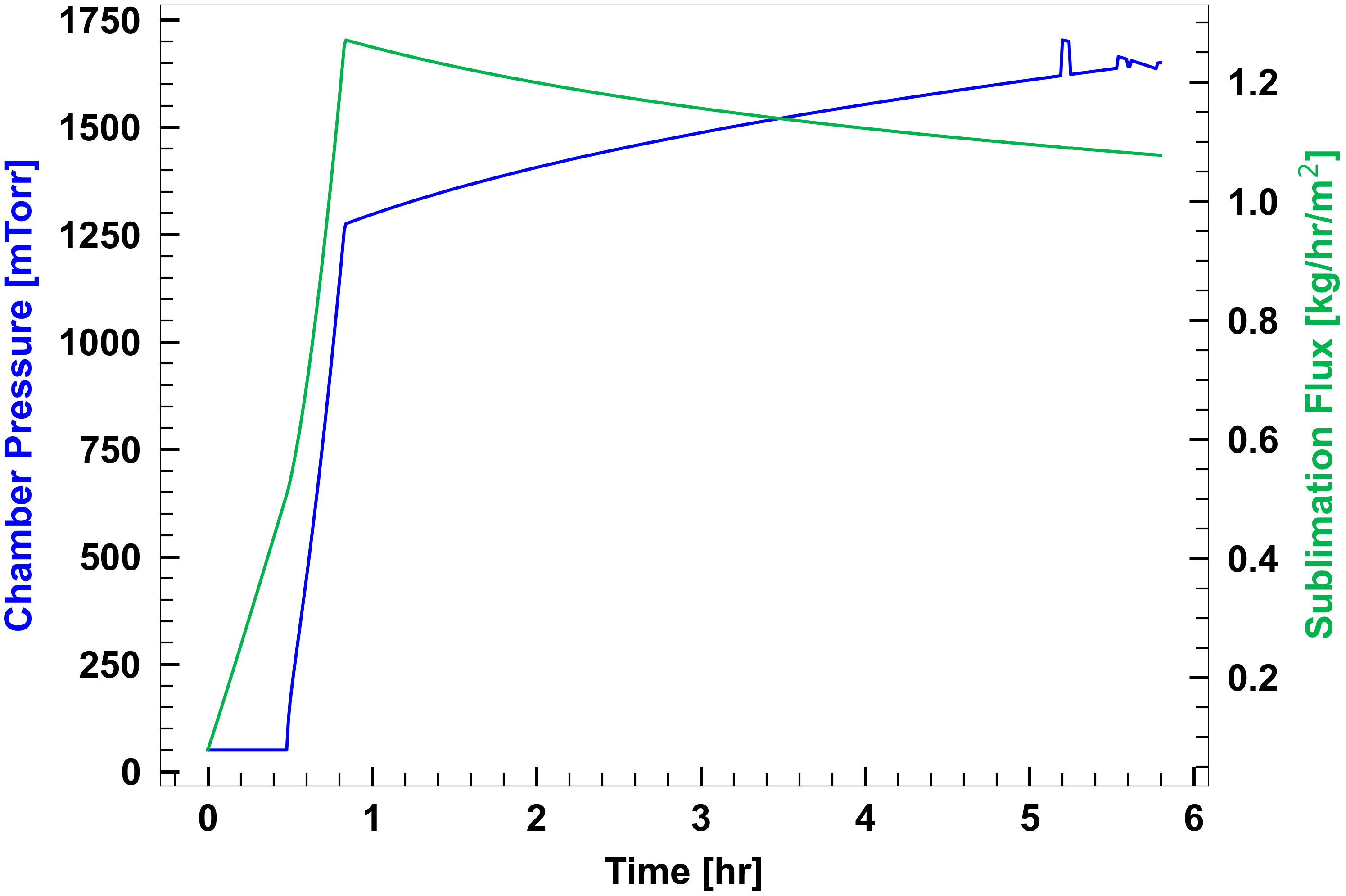
fig = plt.figure(0, figsize=(figwidth, figheight))
ax = fig.add_subplot(1, 1, 1)
plot_styling.axis_style_percdried(ax)
ax.plot(output_table[:, 0], output_table[:, -1], '-k', linewidth=lineWidth, label="Percent Dried")
plt.tight_layout()
# figure_name = 'lyopronto_percentdried_'+current_time+'.pdf'
# plt.savefig(figure_name)
# plt.close()

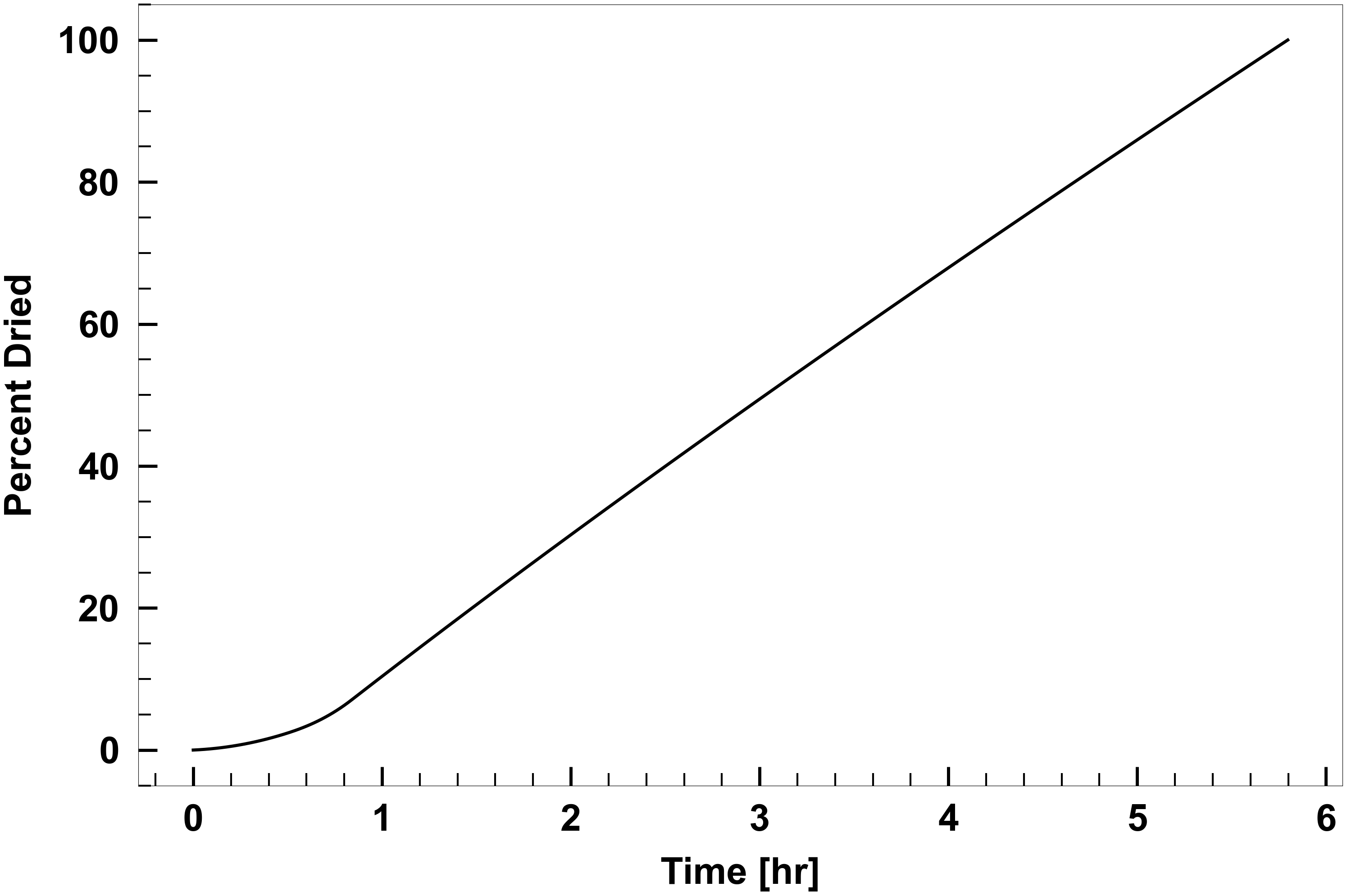
fig = plt.figure(0, figsize=(figwidth, figheight))
ax = fig.add_subplot(1, 1, 1)
plot_styling.axis_style_temperature(ax)
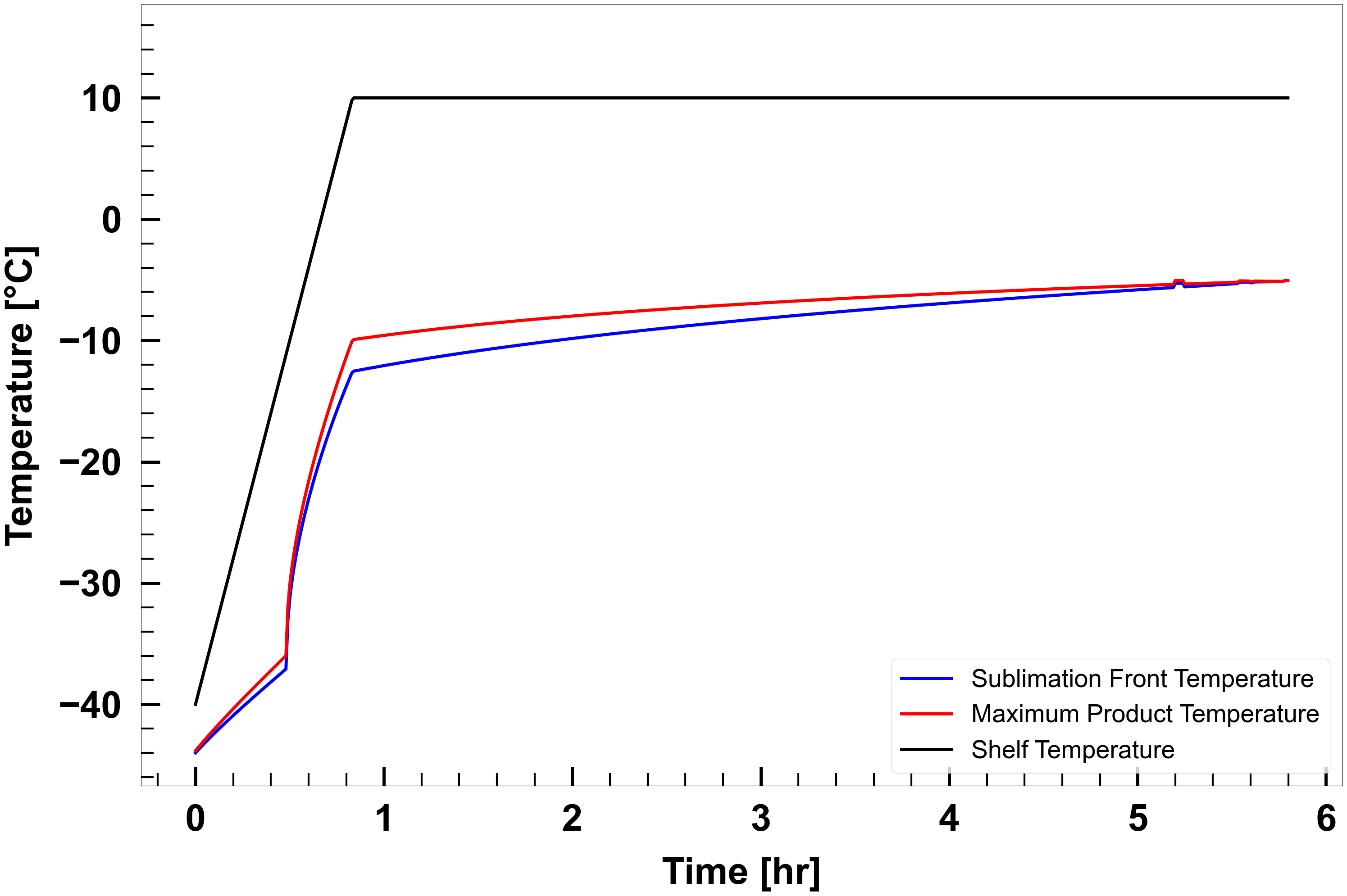
ax.plot(output_table[:, 0], output_table[:, 1], '-b', linewidth=lineWidth, label="Sublimation Front Temperature")
ax.plot(output_table[:, 0], output_table[:, 2], '-r', linewidth=lineWidth, label="Maximum Product Temperature")
ax.plot(output_table[:, 0], output_table[:, 3], '-k', linewidth=lineWidth, label="Shelf Temperature")
plt.legend(fontsize=40, loc='best')
ll, ul = ax.get_ylim()
ax.set_ylim([ll, ul + 5.0])
plt.tight_layout()
# figure_name = 'lyopronto_temperatures_'+current_time+'.pdf'
# plt.savefig(figure_name)
# plt.close()