Extending Fits with New Experimental Data Types

The ExpFitData type is designed to be extensible, so that other types of experimental data beyond those already implemented can be used in the parameter fitting framework. This is done by defining a new subtype of LyoPronto.AbstractExpDatum and implementing the required methods for that type. We will demonstrate this here, with two examples: one which represents a total measurement of $Q_\mathrm{vw-f}$ (heat transfer from vial wall to frozen product) across all of drying, and one which represents a measurement of this heat transfer at specific time points.

using LyoPronto# We will be extending the following functions with new methods, so we need to `import` themimport LyoPronto: AbstractExpDatum, resid_name, obj_exp_datum,    err_exp_datum!# Other packages we needusing LaTeXStringsusing TypedTablesusing Plotsusing StatsPlots: @dfusing Accessors: setproperties# For fittingusing TransformVariablesusing OptimizationOptimJLusing NonlinearSolve

Demonstration case

For demonstration, we will use the model for microwave-assisted lyophilization, with conditions like those in Fitting to Microwave Drying.

vialsize = "6R"rad_i, rad_o = get_vial_radii(vialsize)A_p = π*rad_i^2  # cross-sectional area inside the vialA_v = π*rad_o^2 # vial bottom aream_v = get_vial_mass(vialsize)# Formulation and fillc_solid = 0.05u"g/mL" # g solute / mL solutionρ_solution = 1u"g/mL" # g/mL total solution densityR0 = 1.4u"cm^2*hr*Torr/g"A1 = 16.0u"cm*hr*Torr/g"A2 = 0.01u"1/cm"Rp = RpFormFit(R0, A1, A2)Vfill = 5u"mL"# Heat transferKC = 2.75e-4u"cal/s/K/cm^2"KP = 8.93e-4u"cal/s/K/cm^2/Torr"KD = 0.46u"1/Torr"K_shf = RpFormFit(KC, KP, KD)# Geometryh_f0 = Vfill/A_pm_f0 = Vfill * ρ_solution# RF fit parametersBf = 5.0e8u"Ω/m^2"Bvw = 1.1e7u"Ω/m^2"Kvwf = 22.3u"W/K/m^2"# Controllable inputsf_RF = 8u"GHz"Tsh = RampedVariable(uconvert.(u"K", [-40.0u"°C", 10.0u"°C"]), 0.5u"K/minute")pch = RampedVariable(100u"mTorr")# Total of 10W nominal power, multiplied by 0.54 to account for system lossesP_per_vial = RampedVariable(10u"W"/17 * 0.54) # actual power / vialpo = ParamObjRF((    (Rp, h_f0, c_solid, ρ_solution),    (K_shf, A_v, A_p),    (pch, Tsh, P_per_vial),    (m_f0, LyoPronto.cp_ice, m_v, LyoPronto.cp_gl),    (f_RF, LyoPronto.eppf, LyoPronto.epp_gl),    (Kvwf, Bf, Bvw),))base_sol = solve(ODEProblem(po), LyoPronto.odealg_chunk3)

retcode: Terminated
Interpolation: specialized 4th (Rodas6P = 5th) order "free" stiffness-aware interpolation
t: 69-element Vector{Float64}:
  0.0
  0.1
  0.17061238907357967
  0.2983185121518719
  0.46385893318193705
  0.6897456225251501
  1.0255318480671787
  1.4092808989682446
  1.6666666666666667
  2.056035271752815
  ⋮
 11.089513032354457
 11.089513036334463
 11.08951303884542
 11.089513040495449
 11.089513041536442
 11.089513042220512
 11.089513042652086
 11.089513042935687
 11.089513043071124
u: 69-element Vector{Vector{Float64}}:
 [5.0, 233.14999999999998, 233.14999999999998]
 [4.995438967678863, 236.9087268327139, 238.88875322817526]
 [4.985493377910452, 238.89704151501795, 241.7566089723013]
 [4.956286861999994, 241.40703137582938, 245.3652755477621]
 [4.904694127404679, 243.67174862682367, 248.37639288005465]
 [4.819749480307834, 246.19194724415283, 251.3908698883352]
 [4.671576552815337, 249.67226124856808, 255.36841217453392]
 [4.472835144758677, 253.5189117907176, 259.8132490462152]
 [4.322048560874875, 255.99888596885413, 262.7534389623081]
 [4.079179831009077, 258.3787344504106, 265.8631463307899]
 ⋮
 [2.991106342703887e-9, 264.87680068202536, 313.3174974129898]
 [1.9126818732772043e-9, 265.12404069256445, 313.3174974735967]
 [1.2400523709915088e-9, 264.8768006268917, 313.31749751157315]
 [7.929593835032528e-10, 265.12404066491274, 313.3174975366996]
 [5.141007245258842e-10, 264.8768006080642, 313.3174975524438]
 [3.287449827056194e-10, 265.12404067484545, 313.3174975628607]
 [2.1313582291994867e-10, 264.8768007110776, 313.31749756938797]
 [1.3629104957276827e-10, 265.12404063542135, 313.31749757370653]
 [1.0000015101824183e-10, 264.9304933335642, 313.31749757575506]

Let's take a look at the heat transfer modes over time.

qs = Table(map(base_sol.u, base_sol.t) do u, t    calc_md_Q(u, po, t)end)# LyoPronto provides a slick plot recipe for this, which stacks up the values over time so you can visually compare areast = base_sol.t*u"hr"@df qs areastackplot(t, :Q_shf, :Q_vwf, :Q_RF_f, c=[:red :orange :yellow], labels=[L"Q_\mathrm{sh-f}" L"Q_\mathrm{vw-f}" L"Q_\mathrm{RF-f}"],    xlabel="Time", ylabel="Heat transfer", title="Heat transfer modes over time", unitformat=:square)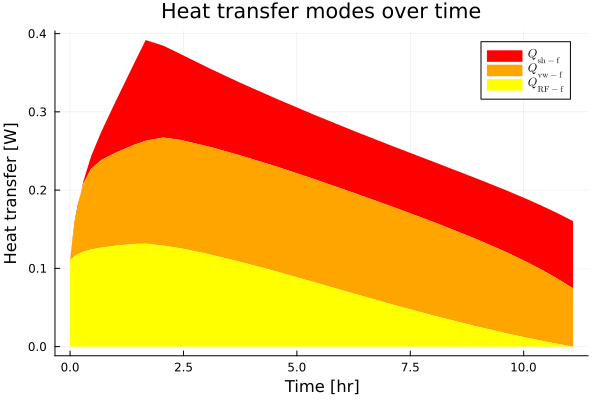

We will use this base solution to create some synthetic experimental data.

First, do a trapezoidal integration to get total $Q_\mathrm{vw-f}$:

t_weights = (vcat(0u"hr", diff(t)) + vcat(diff(t), 0u"hr"))/2total_Qvwf = sum(qs.Q_vwf .* t_weights)

1.3257069146982055 hr W

Now, evaluate $Q_\mathrm{vw-f}$ at specific time points:

t_exp = range(0.0u"hr", stop = 5.0u"hr", step=10u"minute")t_exp_nd = ustrip.(u"hr", t_exp)Q_vwf_exp = [calc_md_Q(base_sol(ti), po, ti).Q_vwf for ti in t_exp_nd]

31-element Vector{Unitful.Quantity{Float64, 𝐋^2 𝐌 𝐓^-3, Unitful.FreeUnits{(W,), 𝐋^2 𝐌 𝐓^-3, nothing}}}:
 0.0 W
 0.06263412844074141 W
 0.09196793884899858 W
 0.10507555679914965 W
 0.11140204955368468 W
 0.11545440654142278 W
 0.11877224489369706 W
 0.1219331022279927 W
 0.12511609707960347 W
 0.12835105327757276 W
 ⋮
 0.13627861968206614 W
 0.13589117458001632 W
 0.1354897281397689 W
 0.13508696776611204 W
 0.1346855180295458 W
 0.13427257488196429 W
 0.13382965152250162 W
 0.1333656753667517 W
 0.1328964834655291 W

Set up the experimental data types

We will define two new types of experimental data, one for the total $Q_\mathrm{vw-f}$ and one for the time series of $Q_\mathrm{vw-f}$.

The TotalQvwf type will represent a single measurement of the total heat transfer from the vial wall to the frozen product over the entire drying process. All it needs to store is a single value of $Q_\mathrm{vw-f}$.

struct TotalQvwf{T} <: AbstractExpDatum    Q_vwf::Tend

Now, we need to define the required methods for this type.

LyoPronto.time_bound_data(::TotalQvwf) = falseLyoPronto.resid_name(::TotalQvwf) = :Qvwf_totalLyoPronto.num_errs(::TotalQvwf) = 1

Define a residual (for nonlinear least squares fitting) and a loss (for optimization-solver least squares fitting).

# Loss function: just returns the errorfunction LyoPronto.obj_exp_datum(sol, dat::TotalQvwf; verbose=false)    q_series = map(sol.u, sol.t) do u, t        calc_md_Q(u, sol.prob.p, t).Q_vwf    end    # Trapezoidal integration over time, really concisely    dt = (x->(vcat(0, x)+vcat(x,0))/2)(diff(sol.t))*u"hr"    qinteg = sum(q_series .* dt) |> u"W*hr"    # Provide some information if requested    verbose && @info "Total Q_vwf: model = $qinteg, exp = $(dat.Q_vwf)"    # The residual is the difference between the model's total Q_vwf and the experimental value    return (qinteg - dat.Q_vwf)^2end# Residual function: fills the error in place in an array, returns number of filled indicesfunction LyoPronto.err_exp_datum!(err_array, i0, sol, dat::TotalQvwf, weight; verbose=false)    q_series = map(sol.u, sol.t) do u, t        calc_md_Q(u, sol.prob.p, t).Q_vwf    end    # Trapezoidal integration over time, really concisely    tweight = (x->(vcat(0, x)+vcat(x,0))/2)(diff(sol.t))*u"hr"    qinteg = sum(q_series .* tweight) |> u"W*hr"    # Provide some information if requested    verbose && @info "Total Q_vwf: model = $qinteg, exp = $(dat.Q_vwf)"    # The residual is the difference between the model's total Q_vwf and the experimental value    # `io` is the last index that was filled into the array    err_array[i0+1] = ustrip(NoUnits, (qinteg - dat.Q_vwf) * weight)    # The number of residuals filled is 1, since this is a single measurement    return 1end

The TimeSeriesQvwf type will represent a series of measurements of $Q_\mathrm{vw-f}$ at specific time points. Since this may or may not be evenly spaced or at the same time points as other measurements, we have fields for a time vector and for a range of indices, but these may be simply set to missing or 1:length(Q_vwf) respectively if not needed. For this example, we will not set those values.

struct TimeSeriesQvwf{T1, T2, T3} <: AbstractExpDatum    Q_vwf::T1    t_range::T2    t::T3end# Set up a constructor which fills in default values when t is in common with other measurementsfunction TimeSeriesQvwf(Q_vwf, t_range=eachindex(Q_vwf); t=missing)    # We could do extra data validation right here    return TimeSeriesQvwf(Q_vwf, t_range, t)end

Main.TimeSeriesQvwf

Now, we need to define the required interface methods for this type.

LyoPronto.time_bound_data(::TimeSeriesQvwf) = true # this data is bound to specific time pointsLyoPronto.resid_name(::TimeSeriesQvwf) = :Qvwf # provide a symbol which will map to weighting in residualLyoPronto.num_errs(q::TimeSeriesQvwf) = length(q.Q_vwf) # indicate how many residuals the data can haveLyoPronto.has_timevec(tq::TimeSeriesQvwf) = !ismissing(tq.t) # indicates whether a separate time vector is providedLyoPronto.nontrivial_t_range(tq::TimeSeriesQvwf) = tq.t_range != eachindex(tq.Q_vwf) # indicates whether the time range is a nontrivial subset of the time vector

Define a loss function (for optimization-solver least squares fitting)

Since this is a time series, we will need to interpolate the model solution to the time points of the experimental data. This is handled internally and managed by the st object, which the obj_exp function will create and pass to this function. You will need to call LyoPronto.exp_time_inds(st) to get the experimental time indices, LyoPronto.model_time_inds(st) to get the model time indices, and length(st) to get the length of the time series. These will be used to index into the experimental data and the model solution, respectively, and the length is used to normalize the residuals so that the residuals are approximately independent of the number of time points which could actually be used in the fit.

# Loss function: just returns the errorfunction LyoPronto.obj_exp_datum(sol, st, dat::TimeSeriesQvwf; verbose=false)    # `st` gets computed internally and used to evaluate the solution only at time points    # where model and experiment are both available    q_series = model_result(sol, st; var=:Q_vwf)    # Provide some information if requested    verbose && @info "Q_vwf:" sum(q_series) LyoPronto.exp_time_inds(st)    # Mean sum of squared differences between model and experimental    return sum(abs2, q_series[LyoPronto.model_time_inds(st)] - dat.Q_vwf[LyoPronto.exp_time_inds(st)])/length(st)end

Define a residual function (for nonlinear least squares fitting)

# Residual function: fills the error in place in an array, returns number of filled indicesfunction LyoPronto.err_exp_datum!(err_array, i0, sol, st, dat::TimeSeriesQvwf, weight; verbose=false)    # The `st` object handles the time alignment between the model solution and the experimental data    q_series = model_result(sol, st; var=:Q_vwf)    # Compute the errors, and normalize by the `sqrt(size of time series)`    # (`sqrt` because if these are squared and summed, it will correspond to above loss)    q_errs = (dat.Q_vwf[LyoPronto.exp_time_inds(st)] .- q_series[LyoPronto.model_time_inds(st)])/sqrt(length(st))    # Total number of experimental data points is the length of the time series    nq = length(dat.Q_vwf)    # Provide some debug info if requested    verbose && @info "Q_vwf errors:" q_errs LyoPronto.exp_time_inds(st)    # Fill in the portion of the error array which corresponds to these data    # with a sentinel value (which indicates the model couldn't evaluate)    err_array[i0 .+ (1:nq)] .= 0.0    # then overwrite the portion where model values are available with the actual errors, weighted appropriately    err_array[i0 .+ LyoPronto.exp_time_inds(st)] .= ustrip.(NoUnits, q_errs * weight)    # Return the number of residuals filled, which is the length of the time series    return nqend

Weighting

For a loss function, the dimensions of the weight need to be the inverse square of the residual dimension, so that the weighted loss is dimensionless. For a residual function, the dimensions of the weight need to be the inverse of the residual dimension, so that the weighted residual is dimensionless.

The keyword argument name to loss_weighting or to residual_weighting should match the symbol returned by resid_name for the data type (as defined above); the default keyword arguments (t, Tf, and Tvw) correspond to resid_name(::EndTimeData), resid_name(::TfData), and resid_name(::TvwSeriesData) or resid_name(::TvwEndData), respectively, so you should also decide appropriate weights for those keyword arguments if you are using those data types in your fitting problem.

To demonstrate, we will construct some example weightings for the two experimental data types we just defined.

single_q_loss_weights = loss_weighting(Qvwf_total = 1.0u"W^-2*hr^-2", Tvw=10.0u"K^-2")multi_q_loss_weights = loss_weighting(Qvwf = 1.0/u"W^2")single_q_resid_weights = residual_weighting(Qvwf_total = 1.0/u"W*hr", Tf=0.5u"K^-1")multi_q_resid_weights = residual_weighting(Qvwf = 1.0*u"W^-1", t=0.01u"hr^-1")

(t = 0.01 hr^-1, Tvw = 1.0 K^-1, Tf = 1.0 K^-1, Qvwf = 1.0 W^-1)

Set up the fitting problem

We will put together two experimental data objects, one for each "measurement" we created above. To demonstrate the results of each separately, we make two ExpFitData objects, but in general any number of experimental data objects can be combined together.

efd1 = ExpFitData(t_exp, TotalQvwf(total_Qvwf))efd2 = ExpFitData(t_exp, TimeSeriesQvwf(Q_vwf_exp))

ExpFitData(31 t pts; TimeSeriesQvwf)

As a toy problem, we will say that we are confident in our estimate of the parameter $K_\mathrm{vw-f}$, but not $B_\mathrm{f}$ and $B_\mathrm{vw}$, so we will adjust $B_\mathrm{f}$ and $B_\mathrm{vw}$ to fit the synthetic experimental data.

We map from dimensionless parameter vector to the named physical parameters using TransformVariables so that the optimization solver can work in an unbounded dimensionless space.

trans = as((;    Bf = TVScale(1e9u"Ω/m^2") ∘ TVLogistic(), #Bracket from 0 to 1e9 Ω/m^2    Bvw = TVScale(1e8u"Ω/m^2") ∘ TVLogistic(), #Bracket from 0 to 1e8 Ω/m^2))

[1:2] NamedTuple of transformations
  [1:1] :Bf → TVScale(1.0e9 Ω m^-2) ∘ as𝕀
  [2:2] :Bvw → TVScale(1.0e8 Ω m^-2) ∘ as𝕀

Optimization problem

We will use the OptimizationOptimJL package to solve the optimization problem, which is a wrapper around the Optim package.

Our optimization functions are as follows, using obj_pd to compute the objective function and the ForwardDiff package for automatic differentiation of the objective function.

obj_single_q = OptimizationFunction((u, p) -> obj_pd(u, p; weights=single_q_loss_weights), AutoForwardDiff())obj_multi_q = OptimizationFunction((u, p) -> obj_pd(u, p; weights=multi_q_loss_weights), AutoForwardDiff())p0 = [-3.0, -3.0] # initial guess in dimensionless spacetransform(trans, p0) # check the values in dimensional space of our initial guess

(Bf = 4.742587317756679e7 Ω m^-2, Bvw = 4.742587317756679e6 Ω m^-2)

It's a good idea at this point to make sure that initial guesses are reasonable. For the microwave model, one quantitative way is to check that the initial guesses satisfy an energy balance on electromagnetic terms:

guessed_po = setproperties(po, transform(trans, p0))LyoPronto.rf_lumcap_EM_violate(guessed_po) # should be false to be reasonable

false

If we had used [0.0, 0.0] as an initial guess, the energy balance would be violated:

guessed_po = setproperties(po, transform(trans, [0.0, 0.0]))LyoPronto.rf_lumcap_EM_violate(guessed_po) # should be false to be reasonable

true

The initial guess gets passed to the optimization problem, along with the transformation, other experimental conditions in po, and the experimental data. Then, we solve the optimization problem using the BFGS algorithm from Optim.

opt1 = solve(OptimizationProblem(obj_single_q, p0, (trans, po, efd1)), Optim.BFGS())

retcode: Success
u: 2-element Vector{Float64}:
 -3.0318551614726807
 -2.4623887764632544

For the time series data, we use the same initial guess and transformation, but with the second experimental data object.

opt2 = solve(OptimizationProblem(obj_multi_q, p0, (trans, po, efd2)), Optim.BFGS())

retcode: Success
u: 2-element Vector{Float64}:
 -0.00010430525937197194
 -2.090750751736804

Let's see how close they got to matching the total $Q_\mathrm{vw-f}$:

(opt1.objective, opt2.objective) # should be close to zero if the fit was good

(5.47891291994186e-19, 1.9712288452582552e-11)

Both very close.

Nonlinear least squares problem

We can also set up a nonlinear least squares problem using the NonlinearSolve package. There are some theoretical advantages to this, since the optimization problem has to take an extra derivative to compute essentially these residuals, but the difficulty for us is in handling the variable number of residuals available from the model (which depends on the model parameters, because those will change total drying time).

Set up a nonlinear least squares problem using a similar approach to the optimization problem, but nls_pd! will be used to compute the residuals; since the length of a cached residual array needs to match the number of experimental data points, LyoPronto provides a convenience constructor for the NonlinearFunction with the signature NonlinearSolve.NonlinearFunction(::ExpFitData; kwargs...).

Here, we will pass a keyword argument badprms to enforce the electromagnetic energy balance we used above to check if our initial guess was reasonable. This can be done for the optimization problem as well, by passing badprms=... in the same place as weights=....

nlf1 = NonlinearFunction(efd1; weights=single_q_resid_weights, badprms=LyoPronto.rf_lumcap_EM_violate)nlf2 = NonlinearFunction(efd2; weights=multi_q_resid_weights, badprms=LyoPronto.rf_lumcap_EM_violate)nls1 = solve(NonlinearLeastSquaresProblem(nlf1, p0, (trans, po, efd1)), LevenbergMarquardt())

retcode: StalledSuccess
u: 2-element Vector{Float64}:
 -3.0
 -3.0

And again for the time series data:

nls2 = solve(NonlinearLeastSquaresProblem(nlf2, p0, (trans, po, efd2)), LevenbergMarquardt())

retcode: StalledSuccess
u: 2-element Vector{Float64}:
 -0.009620119715778669
 -2.0910093538160326

Compare fit results to original data

For all these cases, we can compare the original parameters to the fitted values:

casenames = ["Opt, integrated", "Opt, time", "NLS, integrated", "NLS, time"]cases = [opt1, opt2, nls1, nls2]markers = [:utriangle :dtriangle :ltriangle :rtriangle]guess = transform(trans, p0)plot(xlabel=L"B_\mathrm{f}", ylabel=L"B_\mathrm{vw}", title="Fit results in parameter space", legend=:topleft)scatter!([guess.Bf], [guess.Bvw], label="Initial guess", ms=10, shape=:square)for (name, opt, marker) in zip(casenames, cases, markers)    fit = transform(trans, opt.u)    scatter!([fit.Bf], [fit.Bvw], label=name, ms=10, shape=marker)endscatter!([Bf], [Bvw], label="\"True\"", ms=8, shape=:star5)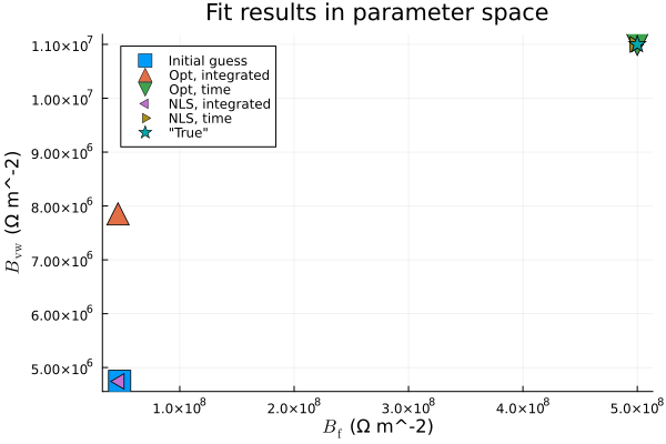

So the fits which had time series data were able to match the true parameters closely (indicated by overlapping markers at the "true" values in the plot above), while the fits which only had total $Q_\mathrm{vw-f}$ did not. The NLS solver did not even move from the initial guess, which suggests that some tolerances might need tweaking, but of course the more productive approach is to give better data.

Next, let's compare the values over time of $Q_\mathrm{vw-f}$ predicted by the model to the synthetic experimental data we created.

t_qvwfs = map(cases) do opt    sol = gen_sol_pd(opt.u, trans, po)    qvwf = map(sol.u, sol.t) do u, t        calc_md_Q(u, po, t).Q_vwf    end    return sol.t*u"hr", qvwfendplot(u"hr", u"W", xlabel="Time", ylabel=L"Q_\mathrm{vw-f}", title="Model predictions vs synthetic experimental data")for (label, (t, qvwf), marker) in zip(casenames, t_qvwfs, markers)    plot!(t, qvwf; label, marker, lw=2, fillto=0, fillalpha=0.1)    @info "check" name t qvwfendscatter!(t_exp, Q_vwf_exp, label="Synthetic experimental data", color=:black)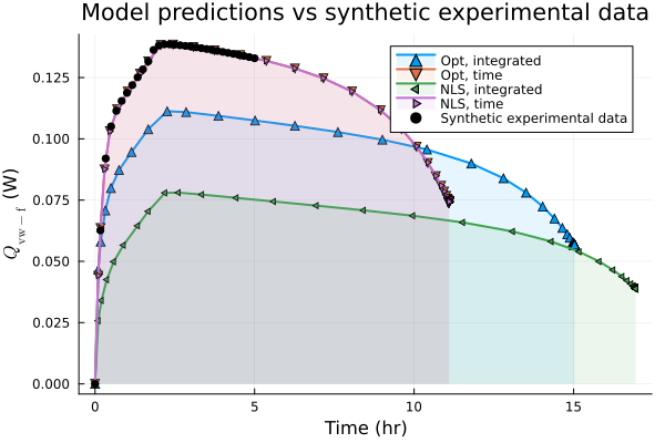

So, both the optimization and nonlinear least squares did a good job of fitting when provided the full time series of $Q_\mathrm{vw-f}$, but unsurprisingly, when the only provided data was matching the total $Q_\mathrm{vw-f}$, the fit doesn't look as good in time, nor does it match the true parameters.

Adding end time to total Qvwf to improve fit

So, as a scientific curiosity, can we get a good overall fit if we match total $Q_\mathrm{vw-f}$ and also match the drying time?

t_end = base_sol.t[end]*u"hr"efd3 = ExpFitData(t_exp, TotalQvwf(total_Qvwf), EndTimeData(t_end))

ExpFitData(31 t pts; TotalQvwf, EndTimeData)

Since single_q_loss_weights already has a weight for t, we don't need a new objective function. It's enough to add the new experimental data.

opt3 = solve(OptimizationProblem(obj_single_q, p0, (trans, po, efd3)), Optim.BFGS())(obj=opt3.objective, Bf=transform(trans, opt3.u).Bf, Bvw=transform(trans, opt3.u).Bvw)

(obj = 1.2652484891947813e-19, Bf = 4.547048884543088e8 Ω m^-2, Bvw = 1.161984474157913e7 Ω m^-2)

Let's see how close it got to matching the time series of $Q_\mathrm{vw-f}$ and the drying time:

sol3 = gen_sol_pd(opt3.u, trans, po)qvwf3 = map(sol3.u, sol3.t) do u, t    calc_md_Q(u, po, t).Q_vwfendt3 = sol3.t*u"hr"plot(u"hr", u"W", xlabel="Time", ylabel=L"Q_\mathrm{vw-f}", title="Model predictions vs synthetic experimental data")plot!(t3, qvwf3; label=L"Both $t_\mathrm{end}$ and total $Q_\mathrm{vw-f}$", marker=:diamond, lw=2, fillto=0, fillalpha=0.1)scatter!(t_exp, Q_vwf_exp, label="Synthetic experimental data", color=:black)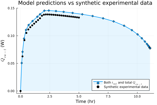

So providing the end time as an additional experimental data point improved things significantly, even though it didn't yield an exact match. This principle will hold in general: the more physical data we can incorporate into the fitting problem, the better our results will be. To put this in machine learning terms, the more features we can provide to the model, the better it will be able to approximate the true physics.

This page was generated using Literate.jl.